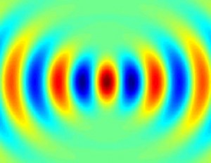
I recently returned to examining transmission / reflection properties of anisotropic planar structures, and I figured that this time around I should do it the Right Way (TM), which boils down to:
1. Take legible notes and
2. Stay the hell away from Mathematica for numerics.
With both of these, I succeeded beautifully. Once again, I have some Matlab code which takes seconds to produce the same results my old Mathematica notebooks would take minutes or hours to compute -- and it's clean, legible, and ran on the first try!
function out = BeamProp1(x,z,kx,kxmask)
    kz0 = sqrt(1 - kx.^2);
    [zz,kk0] = meshgrid(z,kz0);
    fwdPropFieldK = diag(kxmask)*exp(1i.*kk0.*zz);
    clear('zz','kk0'); %free memory
    out = complex(zeros(length(x),length(z)));
    col = 1;
    [xx,kkx] = meshgrid(x,kx);
    for eKZslice=fwdPropFieldK
        [xx,fld] = meshgrid(x,eKZslice); % diff x's are in columns
        eKX = sum(fld.*exp(1i.*xx.*kkx),1).';
        out(:,col) = eKX;
        col=col+1;
    end
end
Couple of notes on the code: first, it does not handle evanescent fields gracefully: if you put evanescent fields (kx > 1) at the origin, they will exponentially grow for z < 0 and will clobber all other features of the plot. Second, the code is fully vectorized -- meaning that it sacrifices memory for speed. The good news is that even though there are 3 vectorized dimensions (x,z,kx), only two of them are put into meshgrid at the same time -- so no 3D matrices to store. Still, expect to have at least a few tens of megs available when dealing with large fields of view.
One Response
Stay in touch with the conversation, subscribe to the RSS feed for comments on this post.
Not sure this is identical but it produces a similar image.
Timing[n = 100;
zlim = 2*Pi*{-1, 2};
zpts = 5*n;
z = N[Range[zlim[[1]], zlim[[2]], (zlim[[2]] - zlim[[1]])/zpts]];
xlim = 10.;
xpts = 3*n;
x = Range[-xlim, xlim, 2*xlim/xpts];
klim = 1.;
kpts = 1*n;
kx = Range[-klim, klim, 2*klim/kpts];
kxmask = Exp[-(Pi/2*kx/klim)^2];
kz0 = Sqrt[1 - kx^2];
fwdPropFieldK =
DiagonalMatrix[kxmask].Exp[I*Transpose[Outer[Times, z, kz0]]];
xxkxx = Exp[I*Transpose[Outer[Times, x, kx]]];
beamMtx = Re[Transpose[xxkxx].fwdPropFieldK];]
This runs in around 0.17 seconds on my machine. Rendering the plot (code below) took around 1.1 seconds.
Timing[ListDensityPlot[beamMtx, ColorFunction -> "Rainbow",MaxPlotPoints -> 200]]
Daniel Lichtblau
Wolfram Research